Decision Tree - Bank Marketing data set (UCI Machine learning repository)

In the last post, we briefly explored the bank marketing data set from UCI Machine learning repository:
https://archive.ics.uci.edu/ml/datasets/Bank+Marketing

In this post, lets explore some simple classification techniques.

Naive Rule: 

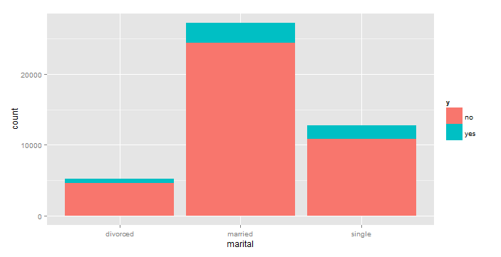
As we mentioned in the previous post, the response rate in this data set is 11.7%. The naive rule here would be to classify all customers as non-subscribers as 88.3% customers in the training set were non-subscribers. Obviously, we are not going to use this for modeling but we may use this later for evaluating the performance of other classifiers. 

My take on performance consideration: 

Before we move to building more models, I want to talk a little bit more about the issue of unequal classes. Here we are dealing with asymmetric classes i.e. it is more important to predict correctly a potential subscriber than a non-subscriber. Why? Because the cost of making a call is likely much lower than misclassifying a potential subscriber as non-subscriber. In other words, we want high sensitivity and low false negative ratio (high negative pred value).

Naive Bayes:

Naive Bayes uses Bayes theorem to compute the (conditional) probability that a record belongs to an output class given a set of predictor variables.

Decision Tree:

We used CART with a cost matrix. We assumed a FN/FP cost ratio of 10:1 in the final model though we also tried other ratios randomly. Anyway, the tree produced with using a cost matrix was clearly much better than without one as we suspected. 

Performance Results:

Gains Chart: 

Using CART decision tree model, we got lifts of 2.9 and 2.3 in the first and second deciles respectively. The lift curve falls apart beyond the 5th decile though, clearly there's a lot of room for improvement.




So, this was my attempt with the bank marketing data set. Hope you are able to take away something positive from it today. 
Please share your thoughts or critique...have discussions if you will. Just don't forget to leave a comment. :)

Exploring Bank Marketing data set (UCI Machine Learning repository)

Bank marketing data set is a very well known data set available at: 
https://archive.ics.uci.edu/ml/datasets/Bank+Marketing . 

The data is related with direct marketing campaigns of a Portuguese banking institution. The marketing campaigns were based on phone calls. Often, more than one contact to the same client was required, in order to assess if the product (bank term deposit) would be ('yes') or not ('no') subscribed. We will work with the older version of the data set (which does not contain the economic parameters). 

Clearly, this is a classification problem and we are interested in identifying the clients that are likely to be subscribers (the yes class).

In this post, we are going to focus on Data Exploration. The next post will discuss some basic classification techniques.

First things first, we looked at data distribution - overall and within the subscriber population. The Response Rate (% subscribers) is 11.70% and like most marketing data sets, this one too is unbalanced.

Some other observations include,

• 52% of the clients who subscribed were married
• 99.02% of the clients who subscribed did not have any credit default
• 63% of subscribers did not have housing loans. 93% did not have a personal loan (Low risk investors)
• 82.61% of subscribers were contacted via cellular
• 71.33% of contacts made were between May and Aug. Within the subscribers, 52.68% of contacts were made between these months.
• 63.98% subscribers were not contacted for past campaigns, so, Poutcome for those is unknown for these subscribers

This data is ordered from May 2008 to Nov 2010 but there is no year variable in the data set, so we added it. We can see that the conversion rate in 2010 was much higher than previous years although the no. of calls reduced.

We also derived and added day of the week variable from the date, month and year variables.

Duration:

When duration = 0, y = no. There are 3 records where duration = 0

Median duration of the last contact is higher for subscribers than for non-subscribers. However, to keep in mind that for a subscriber, duration is not known till the call is over.

Null values: 

There are no null values but some categorical variables have a category called unknown. We will treat these as a valid category for now. 

Reference: 

https://archive.ics.uci.edu/ml/datasets/Bank+Marketing 

Cluster analysis

Cluster analysis, a popular unsupervised learning technique refers to not one but various methods of grouping similar objects together. The aim is to create clusters/groups such that objects in the same group are more similar (a.k.a. intra-cluster homogeneity is high) to each other than to objects in other clusters (inter-cluster heterogeneity is high). 

Cluster analysis is tricky. I heard some people,including some profs say that they don't like cluster analysis, and I can understand why they feel so, but I have come to realize that it may be the most interesting thing I have come across till now. If you know how to do it right, it can help you discover behavioral patterns that you never knew existed. 

In this post, I will explore some basic cluster analysis methods. 

Data set: 

The data set I have used is called Wholesale customers data set from UCI Machine Learning repository. It contains the annual spending of clients of a wholesale distributor on different product categories. I read somewhere that its perhaps one of the best data sets to try for cluster analysis.  Refer the link for more details on the dataset: https://archive.ics.uci.edu/ml/datasets/Wholesale+customers 

Explore data: 

• Channels contain more variability than the regions (Example graph above). Similar patterns emerge for other variables.
• Strong correlation is found in - Grocery & Detergent - 0.92, Milk & Det - 0.66 and Milk & Grocery - 0.73
• Looking at various graphs such as the one above, we can roughly estimate 3 clusters

Hierarchical clustering:

• Different hierarchical clusterings dendrograms roughly categorize data into 3 or 4 groups
• Some observations seem to be separated out consistently (e.g. 86, 87 even though its hard to read here)

K-means: 

Running K-means with size=3,
I wanted to capture more variability in data and found that if we run Kmeans with Grocery, Detergent_Paper and Milk, we can capture 97% variability in data.

Finally, here's my interpretation of the clusters: 
What do you think? Please let me know. Happy learning!

References: 

https://archive.ics.uci.edu/ml/datasets/Wholesale+customers